Joel Carlson Data Scientist
Galvanize - Week 4
One thing that Galvanize does extremely well is tie concepts together. It seems that each week we make more and more use of principles that were explored earlier in the program. This does, however, present a certain pedagogical issue related to how much scaffolding is required to create projects and assignments that push our understanding. For example, this week we worked on building a random forest classifier and were provided a very significant chunk of code to get us started. I spent quite a while just trying to understand the specific implementation rather than the underlying mechanism. On the other hand, being able to read and understand code written by others is certainly also a relevant skill, so perhaps the trade-off here is worthwhile.
This week was our first real introduction to a perspective on machine learning in which interpretation and inference are not necessarily the primary goal. This is not to say that all non-parametric models are uninterpretable, decision trees for example are very much so, but broadly speaking, the fewer assumptions the model makes, the less information it provides (citation needed…).
Day 1
K-nearest neighbors and decision trees were the focus, along with a discussion on the curse of dimensionality. One of the instructors had a very intuitive way to describe the issue - given two points on a line, we know that their distance is just (\(x_2 - x_1)\), now as soon as we add an extra axis on which each of them may vary even slightly, their distance jumps to \(\sqrt{(x_2 - x_1)^2 + (y_2 - y_1)^2}\). We can imagine how quickly this distance blows up as we continue adding dimensions. The more dimensions, the further away each of our ‘neighbors’, and the less meaningful the concept of a neighbor becomes. Short and sweet!
Decision trees were enjoyable and relatively simple to implement. Despite their simplicity, they have a number of favorable features, including that they’re able to handle irrelevant features, they’re computationally cheap, able to model non-linear relationships, and can perform both classification and regression. Unfortunately, they are very weak in terms of accuracy - perhaps now the only real reason to learn about decision trees is to form a base of knowledge on which to build a firmer understanding of random forests.
Day 2
Introduction to bagging (bootstrap aggregating). Continuing to build on techniques we learned earlier the course, we discussed using bootstrapping (taking random samples, with replacement, to simulate a distribution) to create a series of datasets for different weak learners (models with low predictive accuracy). Each of these weak learners on their own may not be able to accurately predict, but by combining their predictions and taking the majority vote (or the average in case of continuous predictions) we may get better results. In the ideal case, where the predictions of each model are independent of the other models, we can write a combination of the models as a binomial distribution:
\[ {n \choose k} p^k (1-p)^{n-k} \]
Where \(n\) is the number of classifiers and \(p\) is the individual classifier strength.
This is how it looks when simulated:
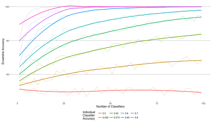
Magic! As can be seen, even very weak classifiers, if uncorrelated with each other, can be combined to make a much stronger classifier. Unfortunately we will never actually have a set of 100 classifiers that are completely uncorrelated with each other, but a dreamer can dream.
Day 3 and 4
On days 3 and 4 we covered support vector classifiers, and gradient boosting. To cover these in the time alotted to lecture we had to do some very serious glossing over of some very serious math. I do understand the difficulty in teaching such complex topics in such a short amount of time, but also wish that we had more time to wrap our heads around some of the concepts. I suppose that is what break week is for.
The assignments were all about practical skills and had us tuning model parameters via cross validation over parameter grids. For me, it was comforting to see that sklearn has much of the model tuning functionality that I relied on heavily while using the R package caret for my research. I wrote a fairly detailed explanation of the process, and also contrasted some of the differences between the python (sklearn) and R (caret) methods for tuning models here.
Day 5
Today was a very different day than most - rather than having lectures and sprints, we instead were given a dataset, a kaggle-like leaderboard, and told to go at it. There are currently two cohorts running, so we paired up into teams of four, with two members from each cohort. I feel it was good for us as a group to get some exposure to the students in the other cohort - we so often inhabit the same spaces, but with the exception of a few, rarely interact.
The dataset given to us was one from a previous kaggle competition which describes a number of attributes of farm vehicles sold at auction, with the goal of predicting sale price. There were many features, and essentially all of the features in the data were categorical. Most of them had huge amounts of missing data (many were greater than 90% NAs), so dealing with that was a top priority. Our strategy went something like:
- Determine which feature to add to our model
- We ran a simple for loop to create bar plots of mean sale price by category in each feature
- Print out the proportion of the column that was NA
- Choose a column based on the criteria that it contained few NA values, and the categories appeared to have significantly different mean sale prices
- Clean the feature
- If the feature was ordinal (such as “size” of vehicle), we encoded it as such
- If the feature was categorical, we made sure to combine redundant categories
- If the feature was binary, we converted it to booleans
- Our method for handling NA values was unique to each column, but heavily subjective
- Add to a model
- We had 3 models that we were adding features into:
- A random forest model
- A gradient boosted tree model
- A linear regression model
- Tune the model parameters
- We used grid search over the parameter space, at larger intervals than we would have liked due to computational constraints
- We used only a subset of the data to tune to save time
- Make predictions
- We ensembled the best performing models using a simple average of the predictions
- Repeat!
- After we were confident that a feature was contributing to our model, we iterated by hunting a new feature, cleaning it, and adding it to the model
It was a very enjoyable day, and a great way to get our hands dirty and really apply some of the toolset we have been working on understanding. Iterating quickly seemed to be the most effective for increasing model accuracy - each time we pulled in a new feature we were doing better and better. Next time around there are some things I wish to improve on, including:
-
Thinking about a more objective/methodical approach for choosing candidate features for the model
-
Using less data to tune the parameters (this was a large time-suck)
-
Grid search over a randomized space, rather than intervals (again, to speed up processing)
-
Iterate faster!