Joel Carlson Data Scientist
Training and Tuning an SVC: R vs Python
Doing data analysis in python after having worked in R for several years makes for some interesting comparisons. It’s impossible to say which is superior, and I have no desire to come down on either side of that debate. I do, however, want to discuss a small subset of differences in something that I consider fairly important: training and tuning machine learning models.
Both languages (R and Python) have well-crafted and thoughtfully designed packages/modules for tuning predictive models. However, the implementations behave and perform in somewhat different ways. In this post I will explore some of these differences. Specifically, I will tune an SVC with a radial basis function kernel by performing a grid search over two parameters, C and gamma (called sigma in the R implementation). Each parameter will be tested using 5-fold cross-validation using a small binary classification dataset. First R, then Python!
Round 1: R
The Data
The data we will be playing with is the same ol’ mtcars dataset, but the specifics of data aren’t the focus today.
#Load the required packages
library(caret); library(ggplot2)
library(ggthemes); library(viridis)

#Load the data
data(mtcars)
dat <- mtcars

#Scale all variables except the response variable
dat[colnames(dat) != 'am'] <- scale(dat[colnames(dat) != 'am'])

#The response column, 'am', must be factor for the SVC
dat$am <- as.factor(dat$am)
Building the Model
With the housekeeping over and done with, we can go ahead and set our model parameters. As stated above, we will perform 5 fold cross validation using the entire dataset for all parameter combinations. The two tunable parameters, C and gamma, will be tuned over \(10^{-1}\) to \(10^3\), and \(10^{-3}\) to \(10^1\), respectively (determined empirically to yield interesting results).
# Set up the 5-fold CV
fitControl <- caret::trainControl(method = "cv",
                                  number = 5)

# Define ranges for the two parameters
C_range =     sapply(seq(-1,3,0.0125), function(x) 10^x)
sigma_range = sapply(seq(-3,1,0.0125), function(x) 10^x)

# Create the grid of parameters
fitGrid <- expand.grid(C     = C_range,
                       sigma = sigma_range)
And that’s it for setting up the parameters. Now we use caret’s extremely convenient train function, which provides a unified api to a huge list of machine learning algorithms:
# Set a random seed for reproducibility
set.seed(825)

# Train the model using our previously defined parameters
Rsvm <- caret::train(am ~ ., data = dat,
                 method = "svmRadial",
                 trControl = fitControl,
                 tuneGrid = fitGrid)
Visualizing the Results
We can examine the results by plotting the data.
Caret provides a lattice plotting method (plot(Rsvm)) and a ggplot2 (ggplot(data=Rsvm)) method for train objects such as Rsvm. I am not fond of the outputs of either, particularly for large tuning grids, so I present the results as a heatmap:
# Note: The below code is simplified - if you run it you will get different results than presented here
res <- data.frame(Rsvm$results)

# Use ggplot to create a heatmap
ggplot(res, aes(x=sigma, y=C)) +
  geom_tile(aes(fill = Accuracy)) +
  labs(x="Gamma", y="C") +
  ggtitle("5-fold Cross-Validation Accuracy")
  scale_fill_viridis() +
  scale_x_log10() +
  scale_y_log10() +
  theme_tufte() +
  theme(axis.text.x = element_text(angle=45)) +
I believe this is a particularly effective way of visualizing a grid search. I find the idea of hyperparameter optimizing as minimizing some function to be very compelling. In this case, since we have only two parameters to optimize, the resulting surface can be easily viewed, and the colours seen as analogous to contours in some 3-dimensional space.
Finally we extract the optimal model parameters using:
Rsvm$bestTune## sigma C
## 53056 0.01333521 11.54782Now let’s move on to python, and contrast some of the differences!
Round 2: Python
import numpy as np
import pandas as pd

from sklearn.preprocessing import StandardScaler
from sklearn.grid_search import GridSearchCV
from sklearn.svm import SVC
import statsmodels.api as sm

import seaborn as sns
import matplotlib.pyplot as plt
from matplotlib.colors import Normalize
%matplotlib inline
#Load up the same dataset as used in R
dat = sm.datasets.get_rdataset("mtcars", "datasets", cache=True).data
As in R, we scale all the predictors. Here we see our first divergences from R: first, as far as a I know, sklearn does not provide a formula interface for creating models, so we split the data into two datasets. Second, rather than calling a function to scale our data as in R, we instantiate a StandardScaler object, and use an internal method on our data:
y = dat.pop('am')
X = StandardScaler().fit_transform(dat)
In R, generic functions have different behaviour for different object classes. A typical example of this is the plot() function, which in my current R session has more than 90 separate object methods (see: methods(plot)).
Building the Model
With the data scaled, we can go ahead and create a parameter grid to tune over:
C_range =     [10**x for x in np.arange(-1,3,0.0125)]
gamma_range = [10**x for x in np.arange(-3,1,0.0125)]

params = {'C':     C_range,
          'gamma': gamma_range}
The next step is to initialize the model, and pass our defined parameters into a GridSearchCV object. No calculation is done in this step:
# Initialize the SVC model
Pysvm = SVC(kernel='rbf')

# Creaste a gridsearch object with our defined parameters
# the cv argument takes input k = folds
svmGS = GridSearchCV(Pysvm, params, scoring='accuracy', cv=5, n_jobs=-1)
We now have another divergence from R. Instead of applying a function (caret::train) to our data, we instantiate a model object and make use of internal methods. Like caret, sklearn has a unified api for doing so (initialize, fit(), predict()):
svmGS.fit(X, y);
Visualizing the Results
Below is a matplotlib visualization that is approximately identical to the one produced with ggplot. Clearly there is less ‘magic’ going on behind the scenes. Perhaps this allows for greater flexibility, certainly it allows for greater frustration…
# Plotting code heavily borrowed from
# http://scikit-learn.org/stable/auto_examples/svm/plot_rbf_parameters.html
# plot the scores of the grid
# grid_scores_ contains parameter settings and scores
# We extract just the scores
n_labs = 40
scores = [x[1] for x in svmGS.grid_scores_]
scores = np.array(scores).reshape(len(C_range), len(gamma_range))

plt.figure(figsize=(16,8) )
plt.imshow(scores,
           interpolation='nearest',
           cmap=plt.cm.viridis,
           norm=MidpointNormalize(vmin=0.6, midpoint=0.75),
           aspect = 0.5)
plt.xlabel('Gamma')
plt.ylabel('C')
plt.colorbar()
plt.xticks(np.arange(0, len(gamma_range), n_labs), np.round(gamma_range[::n_labs],3), rotation=45)
plt.yticks(np.arange(0, len(C_range), n_labs),     np.round(C_range[::n_labs],2))
plt.title('PySVC 5-fold Cross-Validation Accuracy')
plt.grid(False)
plt.show()
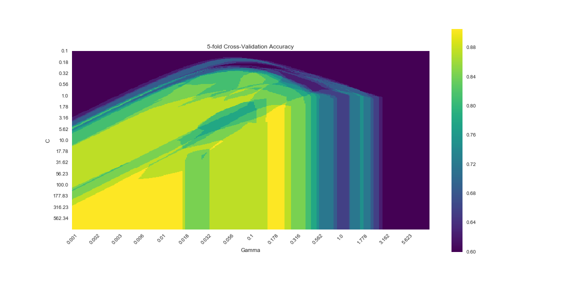
The result looks very similar, but not identical to the results from R. We can extract the best model parameters using:
svmGS.best_params_
##            gamma        C
## 53056 0.21752040 1.631173
Conclusion
We have seen that both languages have fairly simple interfaces to some very powerful techniques. There were differences in both the implementations, which was most obvious in the contrast between the functional caret style, and the more explicitly object-oriented approach taken by sklearn. There were also differences in the final parameters chosen by the two implementations, although we did not explore the reasons here.