Joel Carlson Data Scientist
Exploring Linear Regression Coefficients and Interactions
In this post we will take a very brief look at how to interpret linear regression coefficients. We will then move on to how to visualize interaction terms for continuous variables, and finally how to read interaction coefficients.
Note: unlike most of the other posts on this blog, this post is written in Python.
The first step is to load the usual suspect modules:
import pandas as pd
import numpy as np
import matplotlib.pyplot as plt
import seaborn as sns
import statsmodels.formula.api as smf
%matplotlib inline
Next up is to load the (famous!) dataset:
mtcars = sm.datasets.get_rdataset("mtcars", "datasets", cache=True).data
mtcars.head() #take a quick look
| mpg | cyl | disp | hp | drat | wt | qsec | vs | am | gear | carb | |
|---|---|---|---|---|---|---|---|---|---|---|---|
| Mazda RX4 | 21.0 | 6 | 160 | 110 | 3.90 | 2.620 | 16.46 | 0 | 1 | 4 | 4 |
| Mazda RX4 Wag | 21.0 | 6 | 160 | 110 | 3.90 | 2.875 | 17.02 | 0 | 1 | 4 | 4 |
| Datsun 710 | 22.8 | 4 | 108 | 93 | 3.85 | 2.320 | 18.61 | 1 | 1 | 4 | 1 |
| Hornet 4 Drive | 21.4 | 6 | 258 | 110 | 3.08 | 3.215 | 19.44 | 1 | 0 | 3 | 1 |
| Hornet Sportabout | 18.7 | 8 | 360 | 175 | 3.15 | 3.440 | 17.02 | 0 | 0 | 3 | 2 |
Our goal is to explore how the weight of a car and the number of cylinders are related to the mileage of the car. Additionally, we are interested to know how the weight affects the relationship between the number of cylinders and the mileage. We will answer both of these questions below, but first let’s plot the data to get a sense of how it looks:
sns.lmplot(x='wt', y='mpg', hue='cyl', data=mtcars, fit_reg=False, palette='viridis', size=5, aspect=2.5)
plt.ylabel("Miles per Gallon")
plt.xlabel("Vehicle Weight");
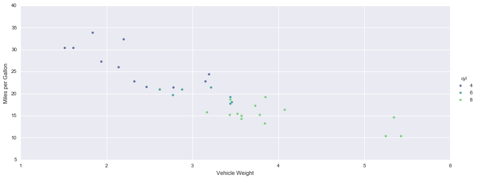
This dataset shows a number of parameters for different cars. The goal is to predict miles per gallon (mpg) given number of cylinders (cyl) and weight (wt). That is, we wish to regress mpg on wt and cyl
Building the Regression Model
Using the statsmodels module we are able to use R style formula input (which includes an intercept term by default):
model = smf.ols(formula='mpg ~ wt + cyl', data=mtcars).fit()
summary = model.summary()
summary.tables[1]
| coef | std err | t | P>|t| | [95.0% Conf. Int.] | |
|---|---|---|---|---|---|
| Intercept | 39.6863 | 1.715 | 23.141 | 0.000 | 36.179 43.194 |
| wt | -3.1910 | 0.757 | -4.216 | 0.000 | -4.739 -1.643 |
| cyl | -1.5078 | 0.415 | -3.636 | 0.001 | -2.356 -0.660 |
The resulting model is written as:
\[ mpg = \beta_0 + \beta_1\cdot{wt} + \beta_2\cdot{cyl} \]
\[ mpg = 39.69 - 3.19\cdot{wt} - 1.51\cdot{cyl} \]
The coefficients of the model can be read as follows:
- For every 1 unit increase in weight, mpg decreases by 3.19 (holding cylinders constant)
- For every 1 unit increase in cylinders, mpg decreases by 1.51 (holding weight constant)
- At 0 weight and 0 cylinders, we expect mpg to be 39.69
- This doesn’t necessarily make sense, noting the maximum value of prestige in the data is 33.9
We also note that the coefficients for wt and cyl have significant p-values (at the common alpha level of 0.05). We interpret the coefficient p-values as the p-value for the hypothesis test where:
- \(H_0\) = The coefficient for this term is zero (null hypothesis)
- \(H_A\) = The coefficient for this term is non-zero (alternative hypothesis)
Thus in both cases we reject the null hypothesis.
Finally, this model has an adjusted \(R^2\) of 0.819 - we will look to improve this with an interaction term.
Modeling the Interaction between wt and cyl
By claiming there may be an interaction between weight and cylinder, we are saying that we believe the relationship between the weight of the vehicle and the mpg is different for vehicles of different numbers of cylinders.
We can add this to our model as follows:
model_interaction = smf.ols(formula='mpg ~ wt + cyl + wt:cyl', data=mtcars).fit()
summary = model_interaction.summary()
summary.tables[1]
| coef | std err | t | P>|t| | [95.0% Conf. Int.] | |
|---|---|---|---|---|---|
| Intercept | 54.3068 | 6.128 | 8.863 | 0.000 | 41.755 66.858 |
| wt | -8.6556 | 2.320 | -3.731 | 0.001 | -13.408 -3.903 |
| cyl | -3.8032 | 1.005 | -3.784 | 0.001 | -5.862 -1.745 |
| wt:cyl | 0.8084 | 0.327 | 2.470 | 0.020 | 0.138 1.479 |
This time, the adjusted \(R^2\) of our model is 0.846, and improvement over the previous value without the interaction term (0.819). We also see that the coefficients on both wt and cyl have changed, but remain significant, and the interaction term is significant. This is evidence that there is an interaction between the variables.
There is no magic in interaction terms, we can see that the term is equivalent to simply multiplying the variables together and using the resulting values as a new predictor:
#Create new variable
mtcars['wt_cyl'] = mtcars.wt * mtcars.cyl

model_multiply = smf.ols(formula='mpg ~ wt + cyl + wt_cyl', data=mtcars).fit()
summary = model_multiply.summary()
summary.tables[1]
| coef | std err | t | P>|t| | [95.0% Conf. Int.] | |
|---|---|---|---|---|---|
| Intercept | 54.3068 | 6.128 | 8.863 | 0.000 | 41.755 66.858 |
| wt | -8.6556 | 2.320 | -3.731 | 0.001 | -13.408 -3.903 |
| cyl | -3.8032 | 1.005 | -3.784 | 0.001 | -5.862 -1.745 |
| wt_cyl | 0.8084 | 0.327 | 2.470 | 0.020 | 0.138 1.479 |
In contrast to the previous formulation, our new formulation is:
\[ mpg = \beta_0 + \beta_1\cdot{wt} + \beta_2\cdot{cyl} + \beta_3\cdot{wt}\cdot{cyl} \]
\[ mpg = 54.31 - 8.66\cdot{wt} - 3.80\cdot{cyl} + 0.81\cdot{wt}\cdot{cyl} \]
But how do we interpret these new coefficients? We say:
-
For every 1 unit increase in weight, mpg decreases by \(8.66\) (holding cylinders at 0)
-
For every 1 unit increase in weight, mpg changes by \(-8.66 + cyl\cdot{0.81}\))
-
For every 1 unit increase in cylinders, mpg decreases by \(3.80\) (holding weight at 0)
-
For every 1 unit increase in cylinders, mpg changes by \(-3.80 + wt\cdot{0.81}\))
-
At 0 weight and 0 cylinders, we expect mpg to be 54.31
- This would be a particularly interesting looking vehicle…
Visualizing Interacting Terms
We can see the interaction by cutting one of the terms in the interaction along it’s median, and then plotting the response variable against the other variable in the interacting pair:
mtcars['cyl_med'] = mtcars.cyl > mtcars.cyl.median()
mtcars['cyl_med'] = np.where(mtcars.cyl_med == False, "Below Median", "Above Median")
sns.lmplot(x='wt', y='mpg', hue='cyl_med', data=mtcars, ci=None, size=5, aspect=2.5);
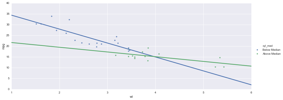
What this plot shows us, is that when the cylinder value is small (i.e. below the median value), the relationship between mpg and wt is strongly negative. Conversely, at higher cylinder values, there is a much weaker relationship between mpg and wt!
In a plot such as this, the larger the difference in slopes, the larger the interaction effect.