Joel Carlson Data Scientist
Galvanize - Week 2
Back in action after a nice weekend rest. Many of the students spent a significant portion of their weekend at the Galvanize campus. The attitude that essentially all of the students share, that of continual learning, is both inspiring and infectious. At this moment I am feeling very good about the environment that Galvanize has curated.
A big positive this week is the integration of the skills we were using last week into our work flow. That is, every assignment we do relies heavily on pandas, numpy, and matplotlib (which I’m still not happy with, but getting better). We dug into probability and statistics this week, and this work, I expect, will serve to ground and motivate much of our future work.
Day 1
Today the lecture material was on stats-101 style probability: coin-flipping, dice rolling, etc. I, along with many of my peers, had seen this material before, which shouldn’t be a surprise: would anyone make the decision to train to become a data scientist before being familiar with the most basic probability and statistics? Occasionally in class I feel as though the lecture material should assume a wider base of knowledge, especially given the promotional material emphasizing that this is not a program for beginners. On a more positive note, the pair programming assignment we completed this afternoon focused much more heavily on using and understanding distributions, which I felt I learned a lot from, and enjoyed very much!
Day 2
Lectures today covered bootstrapping, the central limit theorem, and methods for estimating distribution parameters such as the ‘method of moments’ and ‘maximum likelihood estimation’. Bootstrapping is an excellent method for estimating parameters, see here for a lighthearted introduction to some of the ideas.
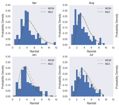
The assignments also logically followed the lectures, and had us estimating the distribution of a given dataset, then using both the method of moments and maximum likelihood estimation to find the optimal shape parameters for the assumed distribution. This produced a wonderful plot showing the differences in the methods:
Later in the afternoon we were tasked with implementing the bootstrap method in python. This exercise really highlighted a difference between R and python that was very interesting for me - to explain I need to digress slightly:
My partner and I chose to first implement the bootstrap (for definition see here by creating an empty array of length 0 (e.g. ret = []), taking a sample from the data, and appending that sample as a list to ret (e.g. ret.append([sample_list]) ).
In R this is a huge no-no - growing a list such as this leads to very slow code, as R needs to make a copy of the ever growing list on each iteration. One way to sidestep this in R is to create a list of the required size (e.g. vector("list", len(n_samples)))) and insert the sample into the pre-allocated list.
I assumed, then, that in python our first method (growing the list) would be slow, but to my surprise it was very fast! Regardless, I wanted to see whether it would be faster to do it the “R way” in python. To this end, I first created a numpy array of the required dimensions (n_samples by sample_length) and looped over the list, inserting into the appropriate slot. Again, to my surprise, this was actually slower than growing the list! Big win for the naive solution!
Day 3
The goal for today was to understand hypothesis testing both qualitatively and quantitatively. I’m glad the former part was emphasized today, as yesterday I felt the qualitative side of the discussion was missing. For example, we discussed the formula for calculating a confidence interval given an appropriate distribution yesterday, but were never given a qualitative intuition for what a confidence interval shows. To say “I have 95% confidence the data is in this interval”, as the name would suggest, would be making an error (more accurately: “This interval will contain the true value 95% of the time”).
Day 4
Power analysis was covered today, with the assignment following the lectures covering A/B testing. In my understanding of the data scientists role in industry, A/B testing is an important part of the toolbox. For this reason, I would have liked to have seen a little more in-depth coverage, and a stronger emphasis on practical interpretation of results. In the pair programming assignment we were ‘designing’ an A/B test, and looking for pitfalls in design, but in reality none of the three of us had a good idea of what we were talking about. It was the blind leading the blind.
Day 5
It was all about that Bayes (I’m so sorry…) today. I can’t believe how much I have been neglecting Bayesian methods in the past, and how fond I find myself after only a day of exposure. But wow. We were looking at the multi-armed bandit problem, which is a variant of A/B testing where, rather than having only a treatment and a control, you have several variants you are looking to test at the same time. There are number of different ways go about assigning participants to each variant in your experiment, and we discussed a number of them. The most naive method would be random assignment, where a participant is, as the name might suggest, put into one of the variants at random - this has issues in that if you have a variant which is clearly inferior, you would continue adding participants to it. No better than simple A/B testing. Surely there is a better way?
Other participant assignment methods we discussed were the epsilon-greedy method (choose a random variant epsilon-percent of the time, otherwise assign to the current best group), the ucb1, and softmax algorithms (which assign participants based on maximization of equations representing the number of times a variant has been played, and the success of that variant thus far). These approaches were nice, and have the potential to create good results. But then, then there was the Bayesian Bandit.
In normal A/B testing, frequentist statistics are often applied - a power analysis is completed to determine the required sample size based on estimated effect size and required power, and then the experiment is done to completion - no peeking at the p-values! The Bayesian Bandit is, put simply, a superior method. The way it works is we assume each variant (bandit) has a beta distribution (defined by two shape parameters, alpha and beta), and we can assume at the outset of the experiment that each variant is equally distributed (i.e. has equivalent shape parameters). The variant the participant is assigned is based on sampling from the set of distributions. After a success in a given variant (a user click, or a product bought), the shape parameters of that variants distribution are adjusted. In this way, as more and mroe successes rack up in the superior distributions, it becomes more likely that we assign participants to them, and more unlikely for participants to be assigned to less performant variants. In practice, the distributions may look like this:
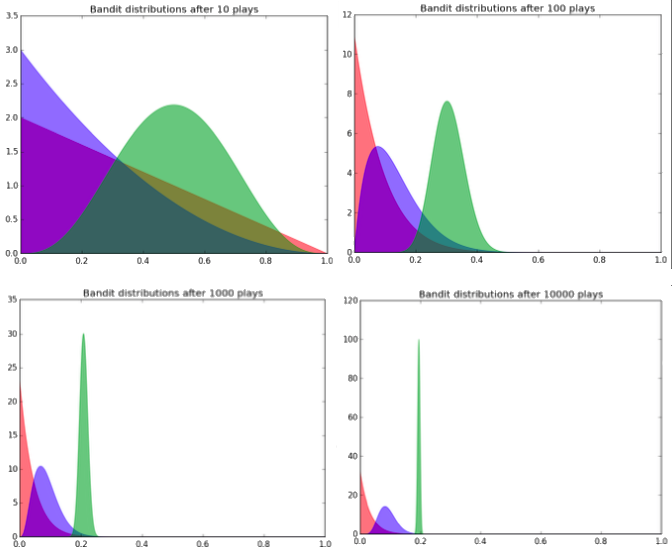
We expect the distributions to converge on their true probability of success (the x-axis). As can be seen, the variant with the highest estimated probability of success (green) has been played much more often than the other two variants (as evidenced by the better defined distribution - it’s parameters have been more finely tuned through the increased probability of being assigned). So I thought that was pretty incredible…