How Good is Texture Analysis at Classification?

Texture analysis is one method of understanding and classifying images. The goal is to quantify relationships between the pixels of a given image. This can be achieved using so called “texture matrices” (described in detail here).

The radiomics package for R provides tools for calculating image texture, and also for calculating first order image features, such as kurtosis, skewness, and mean deviation. We will compare the predictive ability of the first order features to the texture features.

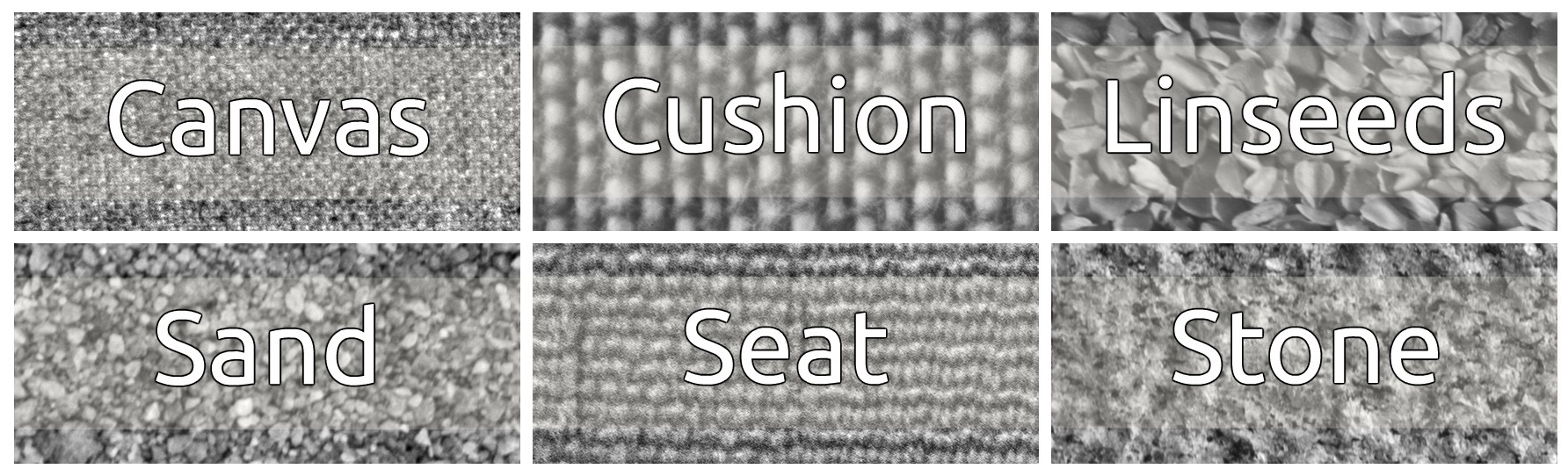
In this post, I will test the efficacy of predictions made using textures features of a sample of images from the Kylberg Texture Dataset V.1.0. The data we will classify contains 40 images from each of the “Canvas”, “Cushion”, “Linseeds”, “Sand”, “Seat”, and “Stone” categories. A representative sample is shown below:

Load Appropriate Packages

library(radiomics); library(ggplot2); library(ggthemes);
library(stringr); library(dplyr); library(caret);
library(png); library(gridExtra); library(viridis)

Calculate Features

Here we calculate the gray level co-occurrence, gray level run-length, and grey level size-zone matrices using the commands glcm(), glrlm(), and glszm(). We then calculate the features of each matrix using the calc_features() command on each matrix, and the image itself (giving the first order features).

For reference, the file structure is such that each of the different image classes has its own folder, and the filename are structured as “class-a-ID” (e.g. “canvas1-a-p017”).

dir <- "~/path/to/the/images/"
lst <- list()

# For each image calculate texture features and add them to a list
for(folder in list.files(dir)){
  for(filename in list.files(paste0(dir,folder))){

    #Load image
    im <- readPNG(paste0(dir,folder,'/',filename))

    #Create texture matrices
    im_glcm <- glcm(im)
    im_glrlm <- glrlm(im)
    im_glszm <- glszm(im)

    #Append to lst
    lst[[filename]] <- cbind(calc_features(im),
                             calc_features(im_glcm),
                             calc_features(im_glrlm),
                             calc_features(im_glszm)
                             )
    }
}

# Convert to data frame
dat <- do.call(rbind, lst)

# Create category label
cat_names <- "canvas|cushion|linseeds|sand|seat|stone"
dat <- dat %>% mutate("Class" = str_match(rownames(dat), pattern = cat_names))

A Quick Peek at the Data

We can gain an understanding of the data by looking at the first two principle components of the data. By splitting the analysis by feature type (i.e. first order, glcm, glrlm, and glszm), we can get some intuition as to which feature type will best separate the classes:

# Function to extract first two principal components given a feature type
get_prcomps <- function(data=dat, feature){
  princomps <- princomp(data[,which(str_detect(colnames(data), feature))])
  data.frame(PC1 = princomps$score[,1],
             PC2 = princomps$score[,2],
             Class = data$Class,
             Feature=feature)
}

# calculate principal components for each feature type
features <- list("calc", "glcm", "glrlm", "glszm")
dat_pca <-do.call(rbind, lapply(features, function(x) get_prcomps(feature=x)))

# There are several extreme outliers in the "calc" principal components,
# here they are removed:
calc_outliers <- which(dat_pca$Feature == "calc" & (dat_pca$PC2 < -1 | dat_pca$PC1 > 100))

# plot PCA analysis
ggplot(data=dat_pca[-calc_outliers,], aes(x=PC1, y=PC2, color=Class)) +
  geom_point(alpha=0.75) +
  facet_wrap(~Feature, scale="free") +
  theme_pander() + scale_color_viridis(discrete=TRUE)

From the plots it is clear that the data is separable; qualitatively moreso by the texture features than by the first order features.

Simple Random Forest Classification

We now turn our attention to building a classification model. We will make some use of the wonderful caret package to take care of splitting the data into training (one third) and testing (two thirds), and also to take care of some very basic model tuning.

set.seed(101)
# Separate into training and test sets
inTrain <- createDataPartition(y=dat$Class, p=0.33, list=FALSE)
training <- dat[inTrain,]
testing <- dat[-inTrain,]

# Train random forest using 5 fold CV
rf_mod <- train(Class ~ . , data=training, method="rf",
                tuneGrid = expand.grid(mtry = 3:15),
                trControl = trainControl(method="repeatedcv",
                                         repeats=20,
                                         number=5))

rf_plot <- ggplot(rf_mod) +theme_pander()
varImp_plot <- ggplot(varImp(rf_mod), top=15) +
  theme_pander() +
  geom_bar(stat = "identity",fill="#3291D4") +
  coord_flip()


# see reproducible doc for confidence interval code
grid.arrange(rf_plot, varImp_plot, ncol=2)

For definitions of the feature suffixes, see here.

Cross validation accuracy is extremely high, hovering in the high 90s. From the variable importance plot we can see that, of the top 10 most important variables used in the random forest, 7 are texture features.

Of course, the more important metric is the test set accuracy:

rf_preds <- predict(rf_mod, testing)

# summarize results
results <- confusionMatrix(rf_preds, testing$Class)
results$table

##           Reference
## Prediction canvas cushion linseeds sand seat stone
##   canvas       26       0        0    0    1     0
##   cushion       0      26        0    0    0     0
##   linseeds      0       0       26    0    0     0
##   sand          0       0        0   26    0     1
##   seat          0       0        0    0   25     0
##   stone         0       0        0    0    0    25

Only 2 were incorrectly classified, for accruacy of 98.7%!

Conclusions

Texture analysis features make excellent input into models for classifying images. Furthermore, the radiomics package makes it simple to calculate them, and get results quickly!