CT Simulation

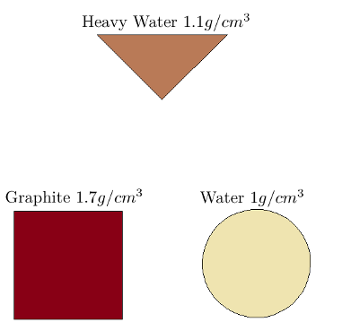
Here I will describe a fun project I did to simulate a first generation CT scan image using MCNPX. The idea was to take a simple geometry: a square, a circle, and a triangle, and create an image using backprojection. The geometry set-up looked like this:

To create an image using backprojection, a projection image must be created by scanning across the geometry. This projection image is really just a measure of the attenuation between the source and detector over a given interval. The geometry is then rotated and the process repeated. To implement this using MCNPX, each interval represents a unique simulation. In this case, I used 100 intervals at 36 angles, resulting in 3600 total simulations. Here is a mockup of the (slightly altered) situation at considerably lower resolution for demonstration purposes:

In the image, the source is a pencil beam originating below the geometry, the red and blue dots represent photons of 100keV interacting with the geometry. The detector scanning across the image at the top measures the incident flux, which can be interpreted as a surrogate for the attenuation between the source and the detector.

Flux Values

The detector outputs a single value at each simulation, which can be plotted against the location of the detector. Here is what the normalized values looks like at each angle:

Each of the values is then converted into a pixel value, and a square image is created:

Laid side to side the images result in a sinogram:

Image Combination

Next, all of the images are rotated to the angle from which they were obtained:

All of the rotated images are then summed together. However, the images must first be darkened such that the maximal sum of pixel values at any given point doesn’t exceed 1, the white value of the image processing software used (EBImage for R). Summing together the rotated images allows us to see the image being iteratively formed:

Reconstructed Image

The last iteration of the image summing gives us the backprojection reconstructed image:

Which looks pretty good! We can even see the how the different densities of the materials changes their visibility in the image! However, the image has a sort of radial blur due to the nature of backprojection. That is, each point in the ‘true’ image is reconstructed as a circular region with decreasing intensity as distance from the center increases.

Filtered Backprojection

To solve the blurring issue the image must be filtered. This is done before reconstruction (ie. summing of the rotated images). The filter kernel used is an approximation of the Sinc function, but with even indices equal to zero. The derivation of the kernel can be found here. Here is a graphical representation of the convolution kernel:

By performing a convolution of the tally values and the kernel we get the following:

From this we can see that the “baseline” value has been converted to be approximately 0.5, which is gray rather than the previous white. Also of note is the emphasis and subsequent de-emphasis of the “edges” in the tally values.

The image reconstructed with this convolution kernel looks like this:

Dynamic Range Adjustment

I found this image to be lacking in dynamic range. A histogram of the normalized pixel values after convolution shows that there are some outliers which squeeze all the other values into a very small range of values.

To remedy this I took a very unsophisticated solution: If the value was greater than 0.8 I set it to 0.8, and if it was less than 0.3 I set it to 0.3.

I then renormalized the convolution values, and the resulting convolution values look like this:

Varying together, the adjusted and unadjusted tally values:

The sinogram of the filtered images:

Final Image

The dynamic range adjusted filtered backprojection image is the final image. The image is significantly less blurry than the original backprojection, and has more contrast than the original filtered image (although it has more artifacts):