Multivariate Regression Modeling

This post will examine multivariate regressions. I have been taking a coursera course about making causal inferences in the social sciences, and while I am not directly involved in social science, the methods are broadly applicable to my own field.

One way to explore the relationships of variables within a dataset is through regressions. One possible relationship between variables is the linear relationship, as shown by mpg vs disp in the mtcars dataset:

The formula given is extremely simple: \[y = a + bx + e\] Where \(y\) is the dependent variable (in this case mpg), and \(x\) is the independent (displacement). The relationship between the two is expressed by the slope term, \(b\), which is interpreted as the change in \(y\) per unit of \(x\), in this case, \(-0.041\) mpg per cubic inch of displacement. The \(a\) term gives the \(y\)-intercept, that is, the value of \(y\) when \(x\) is \(0\), which for the cars data gives the theoretical mpg of a vehicle with \(0\) displacement. The error term is not displayed on the graph.

Multivariate Regressions

Theoretically there is no limit to how many independent variables we wish to include in the model. Let’s consider a different example, perhaps more relatable than technical specs of old cars: The relationship between a students GPA, the years the student spends in school, and their estimated earnings later in life.

In our theoretical model, a student with a higher GPA will generally earn more than a student with a lower GPA. Also, a student who has spent more years studying will have higher earnings than a student who has spent fewer years studying. With these assumptions it is implied that a student with a high GPA, who has spent many years in school will have the highest earnings of all. The converse is also implied, a student who did not study for long, and had a low GPA will have the lowest earnings. Given more than one independent variable, our equation becomes:

\[ y = a + \beta x + \gamma z + \mu \]

In reality this relationship is not so clear cut as the explanation. In a given population very few of the datapoints will actually lie on the plane defined by the model. Many of the data points will be either above or below (ie. high earners with low GPAs, low earners with high GPAs.) This is already taken into account by the error term,\(\mu\), in the equation.

There is also the question of how the independent variables are related to each other. For example, it stands to reason that student who have higher GPAs may go on to study for more years than do their low GPA counterparts.

One way to capture this potential correlation is to look at the relationship between \(x\) and \(z\). In this case again assumed to be linear:

\[ z = \delta + \theta x + \nu \]

If the covariance of \(x\) and \(z\) is not equal to \(0\) then there is evidence that they are related to each other in some way.

\[ cov(z,x) \neq 0 \]

Rearranging and substituting the covariance equation into the regression model returns a linear relationship:

\[ y = a + \beta x + \gamma (\delta + \theta x + \nu) + \mu
\]

Rearranging and collecting like terms gives:

\[ y = a + \gamma \delta + (\beta + \gamma \theta)x + \gamma \nu + \mu \]

\[ y = a + bx + e \]

Where the new \(b = \beta + \gamma \theta\) and the new error term \(e = \gamma \nu + \mu\). We can therefore say that when \(z\) is excluded, \(b\) captures the direct effect of \(x\) and the indirect effect of \(z\) on \(y\). A small caveat, for this to be true \(z\) must have both a direct effect on \(y\), and also be correlated with \(x\) (\(\theta \neq 0\)).

In this case, GPA affects earnings directly, and also indirectly by increasing the years of study, which in turn has a further affect on earnings. In other words, when we manipulate \(x\) (GPA) this causes a direct change in both \(y\) (earnings) and \(z\) (years spent studying), and an indirect change in \(y\) through \(z\). A variable that is causally influenced by an independent variable, and in turn has a causal influence on the dependent variable is known is a mediator. By this definition, years spent studying is a mediator in the relationship between GPA and earnings.

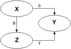
This leads us to a set of equations describing the causal relationships:

1. The DIRECT causal effect of \(x\) controlled for \(z\) is \(\beta\)
2. The INDIRECT effect of \(x\) on \(y\) is \(b - \beta = \gamma \theta\)
3. The TOTAL causal effect, DIRECT (\(\beta\)) + INDIRECT (\(\gamma \theta\)), of \(x\) on \(y\) is \(b\)

These relationships are represented visually in the following figure:

Confounders

In the above we have made the assumption that GPA and time spent studying are the only things that affect earnings. This is clearly not realistic. Without context our results are not guaranteed to be legitimate, which is to say, correlation is not causation.

To illustrate, would anyone ever imagine there being a causal relationship between avalanches and the number of internships at banks?

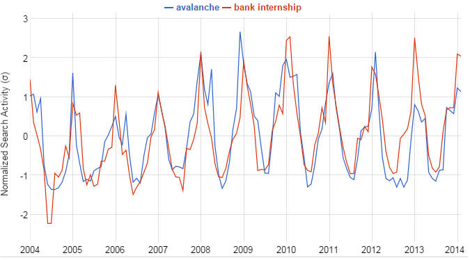
Of course, both of these are seasonal occurrences, and have no causal relationship. Therefore observed effects may be completely, or partly spurious. In the GPA and earnings example perhaps there is another variable. One possibility is innate IQ. Those with a high IQ would presumably have a better GPA, and also be able to achieve higher earnings later in life. If we let \(z\) be innate IQ rather than year spent studying, the directionality of the arrow for \(\theta\) would change in our diagram due to the causal nature of IQ on GPA. This change leads to the equations:

\[y = a + \beta x + \gamma z + e\] \[z = \delta + \theta x + \epsilon\]

Which therefore leads to: \[ y = a + \beta x + \gamma (\delta + \theta x + \epsilon) + e\] \[ \downarrow\] \[y = a + \gamma \delta + (\beta + \gamma \theta)x + e + \gamma \epsilon\]

Where the new constant term, or intercept, is \(a + \gamma \delta\), the slope of \(x\) is \(\beta + \gamma \theta\) and the error term is \(e + \gamma \epsilon\).

So there is some relationship between the variables, and even if \(\beta\) is zero, IQ has an effect on GPA and earnings. If we therefore do not include IQ we may erroneously conclude that better GPA causes higher earnings, because \(\theta\) and \(\gamma\) are non-zero. When the causal effect runs from \(z\) to \(x\) in the diagram we call \(z\) a confounder. By this definition, innate IQ is a confounder.

Controlling for Confounders

We want to control for the effect of the confounder to find the true causal effect of our independent variable on the dependent variable. If the confounder is not present in our data we cannot easily control for it. You don’t know what you don’t know!

We do know, however, that there could be a potential confounder, and given the relationship \[ y = a + \beta x + \gamma z + e\]

we know what the error term looks like if the confounder is unobserved: \(\gamma z + e\). From \[ z = \delta + \theta x + \epsilon\] we can see that \(z\) and \(x\) are correlated. When the two are correlated the effect of \(x\) on \(y\) also involves the effect of the unobserved confounder. It is essential, therefore, that \(x\) and the error term be uncorrelated.

In the absence of confounders we can estimate the slope of the regression for \(y\) vs \(x\) by taking the covariance of \(x\) and \(y\) as follows:

\[cov(x,y) = cov(x, a + bx + e) = cov(x,bx) + cov(x,e) = b*var(x)\] \[b = \frac{cov(x,y)}{var(x)}\]

If the true model is linear, and the error term is uncorrelated with \(x\), then the slope is equal to the causal effect of \(x\) on \(y\). However, in a more realistic situation with confounders, where \(x\) and the error term are correlated, the slope measures both the effect of the confounder, and the effect of \(x\) on \(y\). In this case, the slope from above is measuring the following:

\[\frac{cov(x,y)}{var(x)} = \frac{cov(x, a+ bx + e)}{var(x)} = \frac{cov(x, bx) + cov(x,e)}{var(x)} \] \[= \frac{b*var(x) + cov(x,e)}{var(x)} = b + \frac{cov(x,e)}{var(x)}\]